The introductory vignette covers working with a single study. This one covers many. You assemble a set of studies, then ask what a field reports, what it does not, and how that changes.
Use cases
If you are writing a review, a meta-analysis, or a methods paper, you probably want to say something about how the animals in your corpus were handled, and at the moment that means reading every methods section yourself and keeping notes in a spreadsheet you invented. A shared item set means those notes are comparable with everyone else’s, and the arithmetic is done for you.
Beyond that, a good deal opens up, and most of it is not about reporting at all. A completed sheet records what was done. The actual temperatures, diets, acclimation periods, anaesthetics, killing methods. A set of them is a structured record of husbandry and methods practice, not just a tally of what got mentioned.
What the field actually does. Nobody has a good description of how invertebrates are typically kept and handled in research. What is the modal housing temperature for Drosophila behavioural work? How often is anything used for analgesia in a procedure that would warrant it in a vertebrate? What proportion of field-collected animals are released, and on what reasoning? These are answerable questions that currently are not answered, because the information is scattered through prose.
Methods as moderators. Housing density, photoperiod, acclimation and handling regime all shape outcomes. Extracting them across a corpus gives a meta-analyst covariates rather than unexplained heterogeneity, and may explain why two labs asking the same question of the same species disagree.
Refinement, and whether it spreads. A better practice appears from time to time. A humane endpoint, an anaesthetic protocol, a less damaging trap design. A structured record makes it possible to watch whether it diffuses, how fast, and where it stalls.
Change over time. Both practice and reporting move. Scoring a comparable sample at intervals, or either side of a policy change, turns an impression into a measurement.
Comparison across whatever unit you care about. Taxon, subdiscipline, lab versus field, question type, jurisdiction, funder, decade, institution, journal. Norms differ along all of these, and the differences are often the interesting result rather than a nuisance.
Where the evidence is missing. An item almost nobody reports is either being overlooked or is something the field genuinely does not know how to answer. Both are worth knowing. The first is an advocacy problem, the second a research agenda.
Evidence for policy. Journals, funders and ethics bodies weighing a requirement reasonably ask what it would cost and what it would change. Coverage data answers that far better than a principle does.
Teaching. Handing students a folder of sheets and asking what is missing, or what they would have done differently, is a fast way into both research ethics and methods criticism.
None of this needs the whole literature, or a whole journal. A well-chosen sample of one taxon, one technique or one question is enough to say something.
Compiling a corpus
Three realistic routes, in rough order of how common they will be.
Manual scoring
Read the methods sections and record, for each paper and each item, whether it was reported. This is the main path and will stay that way. Most published work has no INSTAR sheet, and careful reading is still the most reliable way to decide whether an item was genuinely addressed.
Record it as a wide table, one row per paper and one column per
item_id, then hand it to audit_from_matrix().
Section From a scoring table covers
the mechanics.
Worth doing regardless of scale. Score a subset twice, or have a second reader do it, and check agreement before trusting the totals. Reporting is not always a clean yes or no, and the boundary cases are where two readers diverge.
Deposited sheets
Where authors have completed and deposited a sheet, the work is
already done and no reading is required. Point
read_instar() at the folder.
This is the smallest number of studies today and will grow slowly. It is also the reason the sheet is plain text rather than only a figure. A deposited sheet can be read back, a deposited figure cannot.
Assisted extraction
Large language models can be used to pull structured answers out of methods text, and for a corpus of a few hundred papers that is a large saving. It is also easy to do badly. If you go this way, then:
- Validate against hand-scoring. Score a random subset yourself and compare, item by item. Report the agreement. Without this you have numbers of unknown quality.
-
Give the model the item descriptions, not just the
item names.
instar_items$descriptionis written to be exactly this kind of prompt material. - Allow an “uncertain” response as well as yes, no, and not applicable. Forcing a binary choice on ambiguous text manufactures confidence that is not there. Resolve the uncertain ones by hand.
- Report what you did in your methods. Which model and version, the prompt or rubric, how many papers were re-scored by hand, and the agreement you found. This is a methods choice like any other and should be reproducible.
- Feed it the methods section, not the whole paper. Precision improves and cost falls.
The output is the same wide table as manual scoring, so it reaches
audit_from_matrix() the same way. The survey reported in
the INSTAR paper was built this way, and its methods section documents
the model, the rubric, and the hand-validation.
Whichever route you take, the resulting object is the same and everything downstream is identical.
Reading deposited sheets
read_instar() takes a file, a directory, or a vector of
either. Let’s build a small corpus so the examples run.
corpus_dir <- file.path(tempdir(), "supplements")
dir.create(corpus_dir, showWarnings = FALSE)

make_sheet <- function(n_reported, title, journal, doi, housing) {
  # instar_set() takes item_id = value pairs. Building them programmatically
  # means assembling a named list and using do.call().
  ids <- instar_items$item_id[seq_len(n_reported)]
  filled <- stats::setNames(as.list(rep("Reported in the paper", length(ids))),
                            ids)
  filled$env_housing <- housing
  items <- do.call(instar_set, c(list(instar_template()), filled))

  rep <- instar_report(items, paper = list(
    title = title, authors = "Author et al. (2026)",
    journal = journal, doi = doi
  ))
  slug <- gsub("[^A-Za-z0-9]+", "-", doi)
  write_report(rep, file.path(corpus_dir, paste0(slug, ".csv")))
}

invisible(Map(make_sheet,
  n_reported = c(4, 9, 14, 6, 11),
  title      = paste("Study", 1:5),
  journal    = c("J Alpha", "J Alpha", "J Beta", "J Beta", "J Beta"),
  doi        = paste0("10.1234/study", 1:5),
  housing    = c("25 +/- 1 C, 12:12 L:D, 60% RH",
                 "23 C, 14:10 L:D, group housed at 20 per container",
                 "Ambient (18-26 C), natural photoperiod",
                 "25 C, 12:12 L:D, individually housed",
                 "27 +/- 0.5 C, 16:8 L:D, 70% RH")))

list.files(corpus_dir)
#> [1] "10-1234-study1.csv" "10-1234-study2.csv" "10-1234-study3.csv"
#> [4] "10-1234-study4.csv" "10-1234-study5.csv"
Now read them:
corpus <- read_instar(corpus_dir)
#> Reading 5 files...
#>   |                                                                              |                                                                      |   0%  |                                                                              |==============                                                        |  20%  |                                                                              |============================                                          |  40%  |                                                                              |==========================================                            |  60%  |                                                                              |========================================================              |  80%  |                                                                              |======================================================================| 100%
#> ✔ Imported 5 sheets.
corpus
#> <instar_corpus>
#>   5 sheets, INSTAR v1.0
#>   median coverage 56% (range 28-78%)
#>   summary() for per-sheet coverage; instar_audit() for item-level.
A corpus is a named list of reports underneath, so
lapply(), Filter(), [ and friends
all work on it. summary() gives one row per sheet:
summary(corpus)[, c("study", "title", "journal", "reported", "percent_reported")]
#>            study   title journal reported percent_reported
#> 1 10.1234/study1 Study 1 J Alpha        5         27.77778
#> 2 10.1234/study2 Study 2 J Alpha       10         55.55556
#> 3 10.1234/study3 Study 3  J Beta       14         77.77778
#> 4 10.1234/study4 Study 4  J Beta        7         38.88889
#> 5 10.1234/study5 Study 5  J Beta       11         61.11111
When a file will not read
Pointed at a real directory you will meet malformed files. A deleted
column, a semicolon-delimited export, a stray spreadsheet someone left
in the folder. read_instar() does not stop on those. It
warns, skips them, and records what went wrong.
writeLines(c("this,is,not", "an,instar,sheet"),
           file.path(corpus_dir, "junk.csv"))

corpus <- suppressWarnings(read_instar(corpus_dir))
#> Reading 6 files...
#>   |                                                                              |                                                                      |   0%  |                                                                              |============                                                          |  17%  |                                                                              |=======================                                               |  33%  |                                                                              |===================================                                   |  50%  |                                                                              |===============================================                       |  67%  |                                                                              |==========================================================            |  83%  |                                                                              |======================================================================| 100%
#> ✔ Imported 5 sheets.
#> ✖ 1 failed.
attr(corpus, "failed")
#>                                   file
#> 1 /tmp/RtmpRnRBRx/supplements/junk.csv
#>                                                                                                                                                                                                                                                                                     error
#> 1 \033[1m\033[22m\033[34m/tmp/RtmpRnRBRx/supplements/junk.csv\033[39m is missing required columns:\n\033[32mitem_id\033[39m and \033[32mvalue\033[39m.\n\033[36mℹ\033[39m A sheet needs an \033[32mitem_id\033[39m column and a \033[32mreport\033[39m (or \033[32mvalue\033[39m) column.
Getting the other five sheets plus a list of what to go and fix is more useful than getting nothing.
Framework versions
Every sheet records the version it was completed against. A corpus that mixes versions is warned about, because coverage across them is not comparable. An item missing from half the sheets because it did not exist yet is not the same as an item those studies failed to report.
If you do have a mix, split before auditing:
s <- summary(corpus)
v1 <- corpus[s$version == "1.0"]
instar_audit(v1)
From a scoring table
However you produced it, whether by reading papers yourself, a second
coder, or assisted extraction, the shape is one row per paper and one
column per item_id.
scores <- data.frame(
  doi            = c("10.1/a", "10.1/b", "10.1/c", "10.1/d"),
  journal        = c("J Alpha", "J Alpha", "J Beta", "J Beta"),
  year           = c(2024, 2025, 2025, 2026),
  subjects_taxon = c("Y", "Y", "Y", "Y"),
  subjects_n     = c("Y", "N", "N", "Y"),
  env_housing    = c("Y", "Y", "NA", "N"),
  env_field      = c("NA", "NA", "Y", "-"),
  stringsAsFactors = FALSE
)

audit2 <- audit_from_matrix(scores, id = "doi")
#> ℹ 14 framework items not present in `scores` and left out of the audit:
#>   subjects_source, proc_handling, proc_anaesthesia, proc_biosecurity,
#>   ethics_review, ethics_endpoints, ethics_statement, nutrition_diet,
#>   env_acclimation, health_monitoring, health_injury, fate_end,
#>   behaviour_general, and affect_indicators.
summary(audit2)[, c("item", "reported", "applicable", "percent_reported")]
#>                              item reported applicable percent_reported
#> 1 Taxonomic ID, life stage, & sex        4          4        100.00000
#> 2         Sample size & attrition        2          4         50.00000
#> 3    Housing & abiotic conditions        2          3         66.66667
#> 4         Field site & collection        1          1        100.00000
Three things there are worth spelling out.
Cell values are read leniently, because scoring
sheets are made by people. Y, yes,
TRUE, 1 and C all mean reported.
N, no, FALSE and 0
mean not. NA, N/A, - and blanks
mean not applicable. Anything unrecognised warns rather than being
silently counted, so a stray ? or U from an
uncertain call will not slip through as a decision you did not make.
Non-item columns become study metadata.
journal and year are not
item_ids, so they ride along and are immediately available
for grouping:
subset(summary(audit2, by = "year"), item_id == "subjects_n")
#>    year    item_id                    item   domain n_studies reported
#> 2  2024 subjects_n Sample size & attrition Subjects         1        1
#> 6  2025 subjects_n Sample size & attrition Subjects         2        0
#> 10 2026 subjects_n Sample size & attrition Subjects         1        1
#>    applicable percent_reported
#> 2           1              100
#> 6           2                0
#> 10          1              100
Items absent from the table are left out, not counted as unreported. The message above says which. Recording an unscored item as a failure to report would assert something the scoring never checked, which matters if you scored a subset of items deliberately.
Choosing the identifier
id should name a column that identifies every row. If it
does not, you get told rather than finding out later:
incomplete <- data.frame(
  doi = c("10.1/a", "", ""),          # DOI extraction failed for two
  subjects_taxon = c("Y", "N", "Y"),
  stringsAsFactors = FALSE
)
audit3 <- suppressMessages(audit_from_matrix(incomplete, id = "doi"))
#> Warning: Duplicate study identifier in doi: "<blank>".
#> ℹ They have been made unique, so each row still counts as its own study.
#> ! A blank id usually means the column is incomplete rather than that those rows
#>   are duplicates: pick a column that identifies every row.
audit3$n
#> [1] 3
That warns about the blank ids and still counts three studies. It is a real case. In the survey reported in the INSTAR paper, DOI extraction failed for 25 of 150 PDFs, and keying on DOI would have collapsed them into one repeated blank identifier. The fix was to key on a per-file slug instead and keep DOI as metadata.
Auditing
instar_audit() takes a corpus, a scoring table, or a
path directly.
audit <- instar_audit(corpus)
audit
#> <instar_audit>
#>   5 studies, 18 framework items
#>   median study coverage 56% (range 28-78%)
#>
#>   Least often reported:
#>         0%  Injury & mortality
#>         0%  End of study
#>         0%  Behavioural opportunities, enrichment, & disturbance
#>         0%  Indicators & precautionary measures
#>        20%  Acclimation
#>
#>   summary() for all items; summary(by = ) to group; plot() to draw.
summary() gives one row per framework item:
head(summary(audit), 4)
#>           item_id                            item     domain      group
#> 1  subjects_taxon Taxonomic ID, life stage, & sex   Subjects foundation
#> 2 subjects_source        Source & culture history   Subjects foundation
#> 3      subjects_n         Sample size & attrition   Subjects foundation
#> 4   proc_handling  Capture, transport, & handling Procedures foundation
#>   n_studies reported not_reported not_applicable applicable percent_reported
#> 1         5        5            0              0          5              100
#> 2         5        5            0              0          5              100
#> 3         5        5            0              0          5              100
#> 4         5        5            0              0          5              100
Two columns are worth knowing. applicable is the
denominator, which excludes studies that marked the item not applicable,
and percent_reported is reported / applicable.
An item that genuinely does not apply to a study is never counted
against it.
Which items does this literature handle worst?
s <- summary(audit)
head(s[order(s$percent_reported), c("item", "reported", "applicable",
                                    "percent_reported")], 5)
#>                                                    item reported applicable
#> 15                                   Injury & mortality        0          5
#> 16                                         End of study        0          5
#> 17 Behavioural opportunities, enrichment, & disturbance        0          5
#> 18                  Indicators & precautionary measures        0          5
#> 12                                          Acclimation        1          5
#>    percent_reported
#> 15                0
#> 16                0
#> 17                0
#> 18                0
#> 12               20
Grouping
Any study-level column can be a grouping variable. For a corpus read
from sheets that means anything the reserved rows carry, so
journal, doi and version, plus
folder, the directory each sheet came from. For a scoring
table it means any column that was not an item.
by_journal <- summary(audit, by = "journal")
subset(by_journal, item_id == "subjects_taxon")
#>    journal        item_id                            item   domain n_studies
#> 1  J Alpha subjects_taxon Taxonomic ID, life stage, & sex Subjects         2
#> 19  J Beta subjects_taxon Taxonomic ID, life stage, & sex Subjects         3
#>    reported applicable percent_reported
#> 1         2          2              100
#> 19        3          3              100
folder is the useful one when a corpus is filed into
directories that mean something. Read recursively and the structure
comes through:
corpus <- read_instar("corpus/", recursive = TRUE)
summary(instar_audit(corpus), by = "folder")
Per-study coverage
audit$studies is one row per study, which is what you
want for questions about papers rather than items:
Plotting
plot(audit)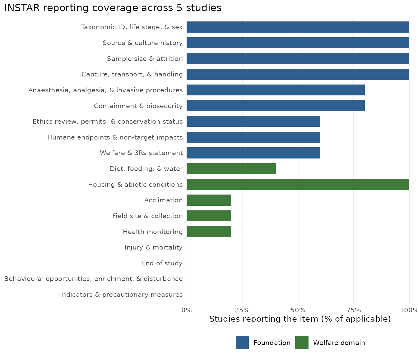
autoplot() returns the ggplot object instead of drawing
it, so you can modify it before rendering.
plot(audit, by = "journal") facets.
Beyond coverage, to what the studies actually did
Coverage tells you whether an item was addressed. The sheet also carries what was said, which for most of the questions in Use cases is the part you want. Each report keeps the text in its items table, so pulling one item across a corpus is a one-liner:
d <- as.data.frame(corpus)

subset(d, item_id == "env_housing" & status == "reported",
       select = c(study, value))
#>             study                                             value
#> 11 10.1234/study1                     25 +/- 1 C, 12:12 L:D, 60% RH
#> 29 10.1234/study2 23 C, 14:10 L:D, group housed at 20 per container
#> 47 10.1234/study3            Ambient (18-26 C), natural photoperiod
#> 65 10.1234/study4              25 C, 12:12 L:D, individually housed
#> 83 10.1234/study5                    27 +/- 0.5 C, 16:8 L:D, 70% RH
From there it is ordinary text work. Parse temperatures out, tabulate photoperiods, count how many housed animals individually. The framework does not standardise the content, deliberately, since forcing husbandry into fixed fields would lose more than it gained. It does guarantee that the housing description sits in the housing row of every sheet, which is most of the battle.
The same applies to any item. fate_end across a corpus
tells you how often animals are released, killed, or kept.
proc_anaesthesia tells you what is actually used, and how
often nothing is. ethics_review tells you how often review
applied at all, and what reasoning was offered when it did not.
as.data.frame() on a corpus gives one row per study per
item, carrying the paper’s details alongside, so grouping and filtering
are ordinary data frame work.
str(d, vec.len = 2)
#> 'data.frame':    90 obs. of  10 variables:
#>  $ study  : chr  "10.1234/study1" "10.1234/study1" ...
#>  $ title  : chr  "Study 1" "Study 1" ...
#>  $ doi    : chr  "10.1234/study1" "10.1234/study1" ...
#>  $ journal: chr  "J Alpha" "J Alpha" ...
#>  $ item_id: chr  "subjects_taxon" "subjects_source" ...
#>  $ item   : chr  "Taxonomic ID, life stage, & sex" "Source & culture history" ...
#>  $ domain : chr  "Subjects" "Subjects" ...
#>  $ group  : chr  "foundation" "foundation" ...
#>  $ status : chr  "reported" "reported" ...
#>  $ value  : chr  "Reported in the paper" "Reported in the paper" ...